── Conflicts ────────────────────────────────────────── tidyverse_conflicts() ──
✖ dplyr::filter() masks stats::filter()
✖ dplyr::lag()    masks stats::lag()
ℹ Use the conflicted package (<http://conflicted.r-lib.org/>) to force all conflicts to become errors
library(tidycensus) # Tidily interact with the US Censuslibrary(maps) # Some basic maps
Attaching package: 'maps'

The following object is masked from 'package:purrr':

    map
library(sf) # Make maps in ggplot
Linking to GEOS 3.11.0, GDAL 3.5.3, PROJ 9.1.0; sf_use_s2() is TRUE
library(tigris) # Talk to the Census's TIGER data
To enable caching of data, set `options(tigris_use_cache = TRUE)`
in your R script or .Rprofile.
library(colorspace) # Paletteslibrary(nycdogs) # New York City dog license data
Mapping
Joining tables, and using geom_polygon()
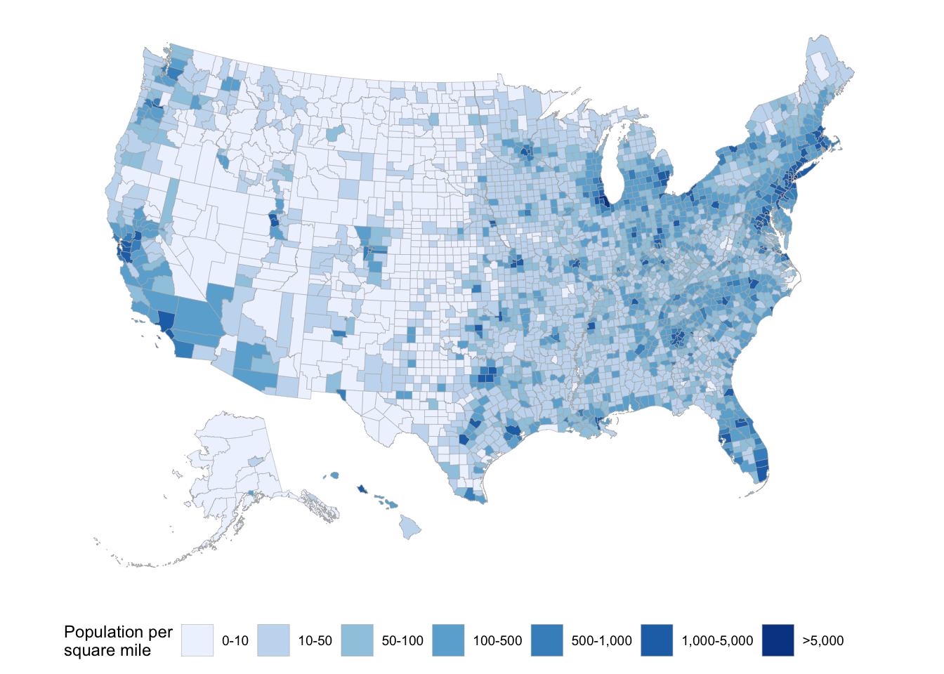
Remember, we use geom_polygon() as a kind of illustration of what’s happening conceptually. It is not our go-to method for mapping.
# Create a theme that turns off most of the stuff ggplot usually printstheme_map <-function(base_size=9, base_family="") {require(grid)theme_bw(base_size=base_size, base_family=base_family) %+replace%theme(axis.line=element_blank(),axis.text=element_blank(),axis.ticks=element_blank(),axis.title=element_blank(),panel.background=element_blank(),panel.border=element_blank(),panel.grid=element_blank(),panel.spacing=unit(0, "lines"),plot.background=element_blank(),legend.position ="inside",legend.justification =c(0,0),legend.position.inside =c(0,0) )}head(county_map)
  [1]  1.15  0.23    NA  0.21  1.13  1.38    NA  0.80  0.89  1.39  0.92    NA
 [13]  0.38  0.84  0.64  0.19  0.56  1.28  0.68    NA    NA  1.52  0.73  0.20
 [25]  0.74  1.37    NA  0.80  0.43  0.90  0.17  1.05  0.52  0.66  0.29  0.30
 [37]  0.47  0.44  0.64  0.51  0.31  0.78  0.31  0.82  0.33  0.53  0.37  0.31
 [49]  0.30  1.11  1.64  0.78  1.30  0.66  0.19  0.33  0.33  0.77  0.85  0.83
 [61]  1.04  0.64  0.36  0.43  1.24  0.83  1.37  0.37  0.45  0.25  1.85  0.29
 [73]  0.57  0.90  1.20  0.18  1.29  0.67  1.19  0.67  0.49  1.10    NA  0.77
 [85]    NA  1.51  0.91  1.22    NA  1.94  1.02  1.37  1.23  1.88  0.75  0.96
 [97]  0.64  0.56  0.80  1.92  0.30  1.87  1.10  0.69  0.59  3.41  0.64  3.06
[109]  0.55  3.83    NA    NA  1.97  3.38  4.30  3.25  1.17  3.74  2.68  0.43
[121]  3.54  2.35  1.36  1.97  0.55  2.31  2.71  3.69  2.33  4.57  1.71  0.83
[133]  3.08  1.32  4.02  0.11  4.71    NA  4.58  0.20  2.35  4.58  1.79  0.31
[145]  0.60  4.58  4.58    NA  0.90  1.01  0.98    NA  0.32  0.83  1.05  0.60
[157]  0.98  1.03    NA  0.19  0.11  0.37  0.65  0.35  0.33  0.07  0.45  1.26
[169]  0.09  1.08  0.83  0.46  0.09  0.95    NA  0.52  0.64  0.77  0.59    NA
[181]  0.72  0.09  0.64  0.68  0.09  0.43    NA  0.81  0.26    NA  0.60  0.58
[193]  0.90  2.26    NA    NA    NA    NA    NA    NA    NA 50.00    NA  2.89
[205]    NA    NA    NA    NA    NA    NA    NA    NA    NA    NA    NA    NA
[217]    NA    NA    NA    NA    NA    NA    NA    NA    NA    NA    NA    NA
[229]    NA    NA    NA    NA    NA    NA    NA    NA    NA    NA  1.51    NA
[241]    NA    NA    NA    NA    NA    NA    NA 50.00    NA    NA    NA    NA
[253]    NA    NA    NA    NA  0.75  1.68  1.64  2.57    NA  5.67
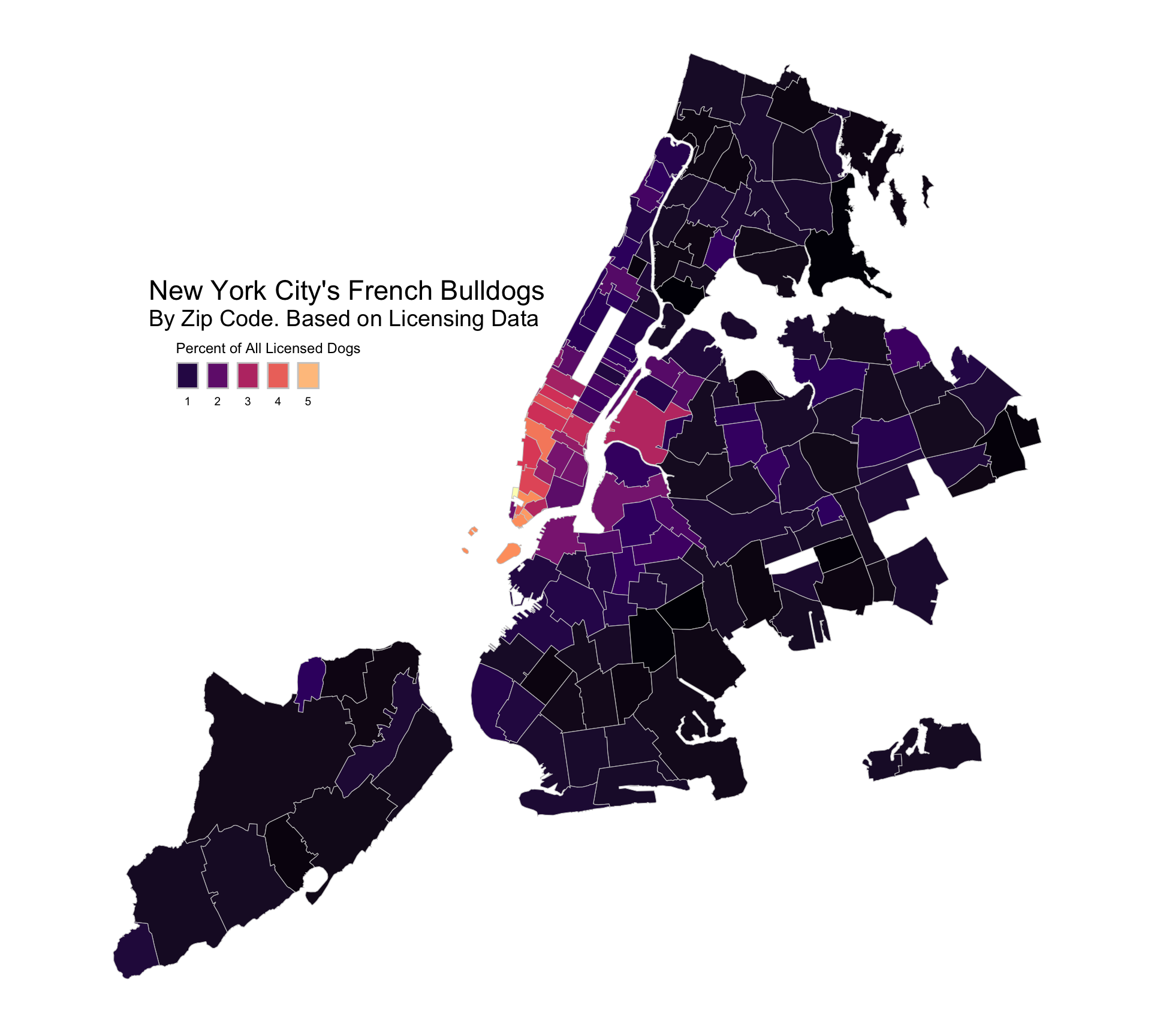
fb_map |>filter(n >1) |>ggplot(mapping =aes(fill = pct)) +geom_sf(color ="gray80", size =0.1) +scale_fill_viridis_c(option ="A") +labs(fill ="Percent of All Licensed Dogs") +# This next bit is a hack--we're just positioning the boxes# relative to the latitude/longitude coordinatesannotate(geom ="text", x =-74.145+0.029, y =40.82-0.012, label ="New York City's French Bulldogs", size =6) +annotate(geom ="text", x =-74.1468+0.029, y =40.8075-0.012, label ="By Zip Code. Based on Licensing Data", size =5) +theme_nymap() +guides(fill =guide_legend(title.position ="top", label.position ="bottom",keywidth =1, nrow =1))
Simple feature collection with 262 features and 15 fields
Geometry type: POLYGON
Dimension:     XY
Bounding box:  xmin: -74.25576 ymin: 40.49584 xmax: -73.6996 ymax: 40.91517
Geodetic CRS:  WGS 84
# A tibble: 262 × 16
   objectid zip_code po_name     state borough st_fips cty_fips bld_gpostal_code
      <int>    <int> <chr>       <chr> <chr>   <chr>   <chr>               <int>
 1        1    11372 Jackson He… NY    Queens  36      081                     0
 2        2    11004 Glen Oaks   NY    Queens  36      081                     0
 3        3    11040 New Hyde P… NY    Queens  36      081                     0
 4        4    11426 Bellerose   NY    Queens  36      081                     0
 5        5    11365 Fresh Mead… NY    Queens  36      081                     0
 6        6    11373 Elmhurst    NY    Queens  36      081                     0
 7        7    11001 Floral Park NY    Queens  36      081                     0
 8        8    11375 Forest Hil… NY    Queens  36      081                     0
 9        9    11427 Queens Vil… NY    Queens  36      081                     0
10       10    11374 Rego Park   NY    Queens  36      081                     0
# ℹ 252 more rows
# ℹ 8 more variables: shape_leng <dbl>, shape_area <dbl>, x_id <chr>,
#   geometry <POLYGON [°]>, breed_rc <chr>, n <int>, freq <dbl>, pct <dbl>
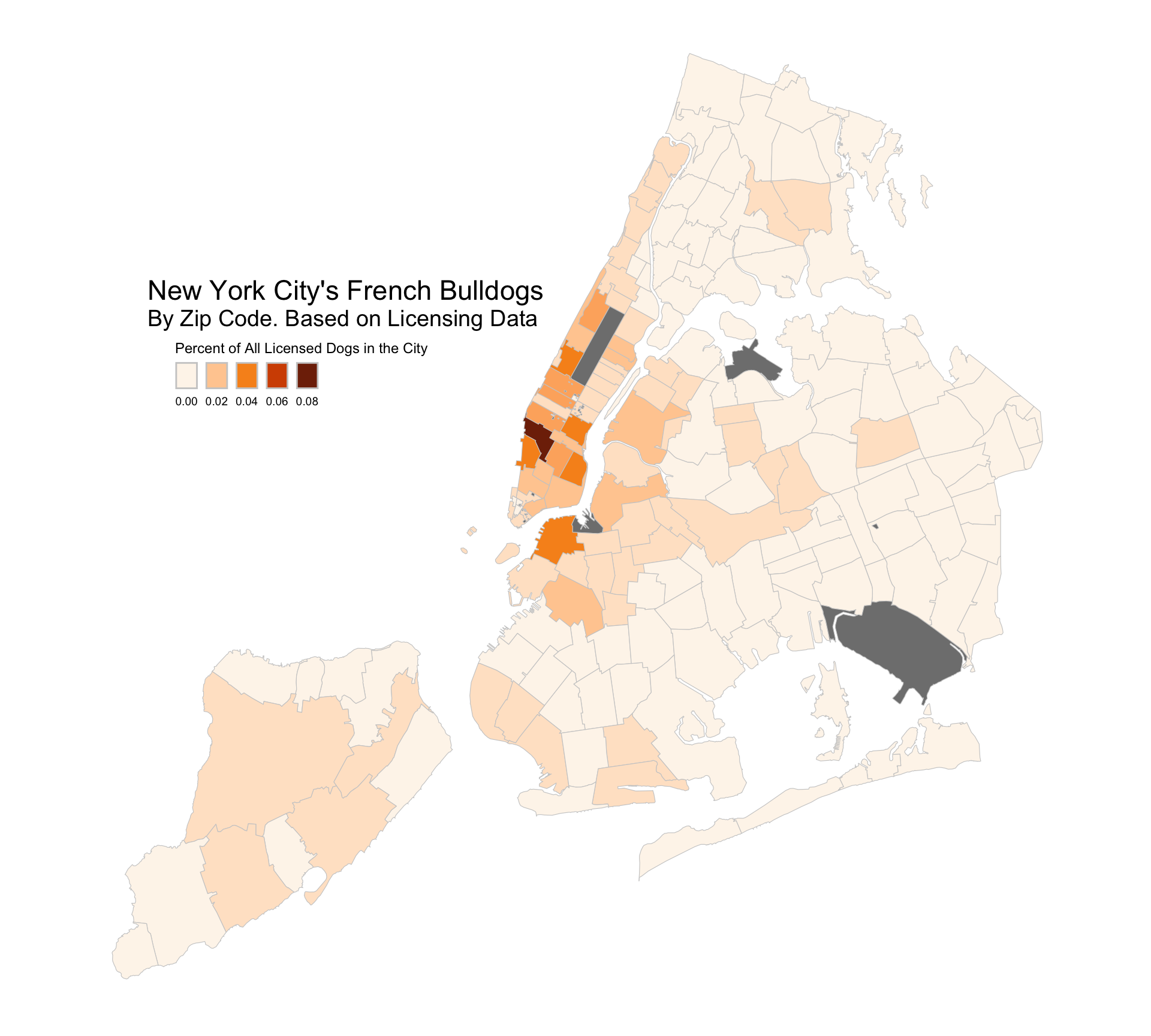
fb_map |>ggplot(mapping =aes(fill = pct)) +geom_sf(color ="gray80", size =0.1) +scale_fill_continuous_sequential(palette ="Oranges") +labs(fill ="Percent of All Licensed Dogs in the City") +annotate(geom ="text", x =-74.145+0.029, y =40.82-0.012, label ="New York City's French Bulldogs", size =6) +annotate(geom ="text", x =-74.1468+0.029, y =40.8075-0.012, label ="By Zip Code. Based on Licensing Data", size =5) +theme_nymap() +guides(fill =guide_legend(title.position ="top", label.position ="bottom",keywidth =1, nrow =1))
Census data
Population components example
# From the Census. You will need a census API key and the tidycensus packageus_components <-get_estimates(geography ="state", product ="components", vintage =2019)
us_components
# A tibble: 624 × 4
   NAME           GEOID variable  value
   <chr>          <chr> <chr>     <dbl>
 1 Mississippi    28    BIRTHS    35978
 2 Missouri       29    BIRTHS    71297
 3 Montana        30    BIRTHS    11618
 4 Nebraska       31    BIRTHS    25343
 5 Nevada         32    BIRTHS    35932
 6 New Hampshire  33    BIRTHS    12004
 7 New Jersey     34    BIRTHS    99501
 8 New Mexico     35    BIRTHS    23125
 9 New York       36    BIRTHS   222924
10 North Carolina 37    BIRTHS   119203
# ℹ 614 more rows
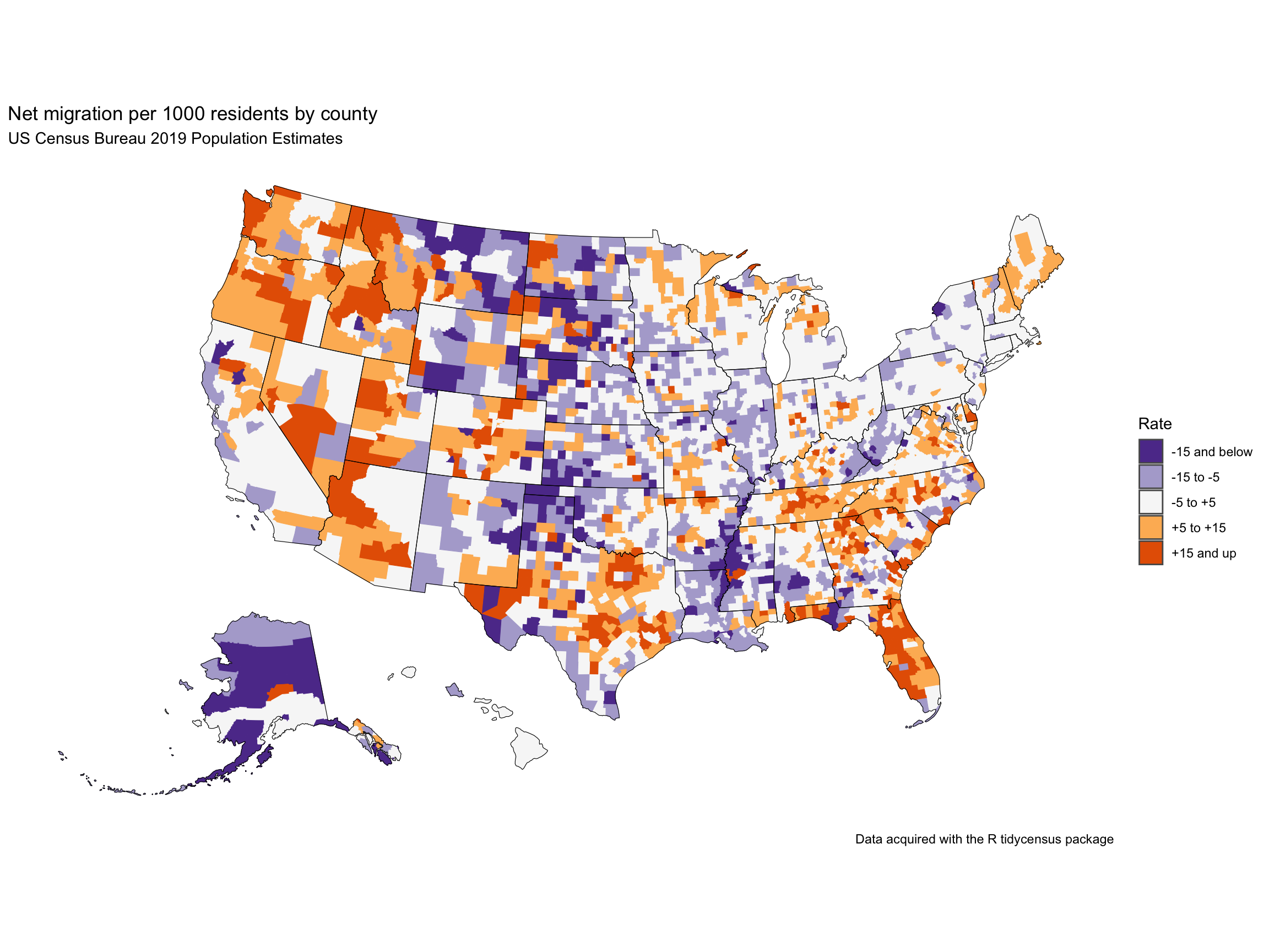
net_migration <-get_estimates(geography ="county",variables ="RNETMIG",year =2019,geometry =TRUE,resolution ="20m") |>shift_geometry() # puts Alaska and Hawaii in the bottom left
order <-c("-15 and below", "-15 to -5", "-5 to +5", "+5 to +15", "+15 and up")net_migration <- net_migration |>mutate(groups =case_when( value >15~"+15 and up", value >5~"+5 to +15", value >-5~"-5 to +5", value >-15~"-15 to -5",TRUE~"-15 and below" )) |>mutate(groups =factor(groups, levels = order))net_migration
Simple feature collection with 3142 features and 5 fields
Geometry type: GEOMETRY
Dimension:     XY
Bounding box:  xmin: -3112200 ymin: -1697728 xmax: 2258154 ymax: 1558935
Projected CRS: USA_Contiguous_Albers_Equal_Area_Conic
# A tibble: 3,142 × 6
   GEOID NAME                   variable  value                  geometry groups
 * <chr> <chr>                  <chr>     <dbl>        <MULTIPOLYGON [m]> <fct>
 1 29227 Worth County, Missouri RNETMIG   -8.91 (((114835.6 345071.6, 12… -15 t…
 2 31061 Franklin County, Nebr… RNETMIG  -14.4  (((-267685.1 323958.5, -… -15 t…
 3 36013 Chautauqua County, Ne… RNETMIG   -3.54 (((1324221 647717.4, 133… -5 to…
 4 37181 Vance County, North C… RNETMIG   -3.25 (((1544260 32202.52, 154… -5 to…
 5 47183 Weakley County, Tenne… RNETMIG   -1.02 (((625934.5 -98887.34, 6… -5 to…
 6 44003 Kent County, Rhode Is… RNETMIG    2.29 (((1977965 726702.3, 200… -5 to…
 7 08101 Pueblo County, Colora… RNETMIG    6.15 (((-783174.5 122269, -77… +5 to…
 8 17175 Stark County, Illinois RNETMIG  -10.6  (((500559 424779.4, 5102… -15 t…
 9 29169 Pulaski County, Misso… RNETMIG    4.42 (((312851.7 46166.36, 31… -5 to…
10 19151 Pocahontas County, Io… RNETMIG  -12.2  (((88185.95 606331.9, 12… -15 t…
# ℹ 3,132 more rows
# So we can draw state boundaries (our migration data is at the county level)state_overlay <- tigris::states(cb =TRUE,resolution ="20m") |>filter(GEOID !="72") |>shift_geometry()ggplot() +geom_sf(data = net_migration, mapping =aes(fill = groups, color = groups), size =0.1) +geom_sf(data = state_overlay, fill =NA, color ="black", size =0.1) +scale_fill_brewer(palette ="PuOr", direction =-1) +scale_color_brewer(palette ="PuOr", direction =-1, guide ="none") +coord_sf(datum =NA) +theme_minimal() +labs(title ="Net migration per 1000 residents by county",subtitle ="US Census Bureau 2019 Population Estimates",fill ="Rate",caption ="Data acquired with the R tidycensus package")
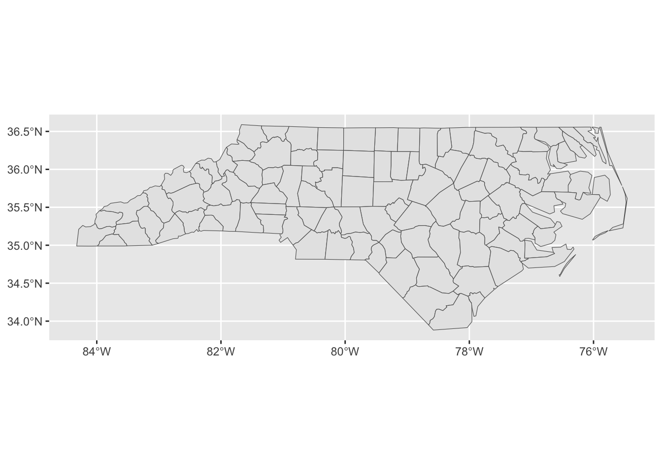
Simple Features work smoothly with dplyr grouping and summarizing
## This shapefile comes built-in to the sf package as an example. Here## we extract it and put it in an objectnc <-st_read(system.file("shape/nc.shp", package ="sf"), quiet = T)nc
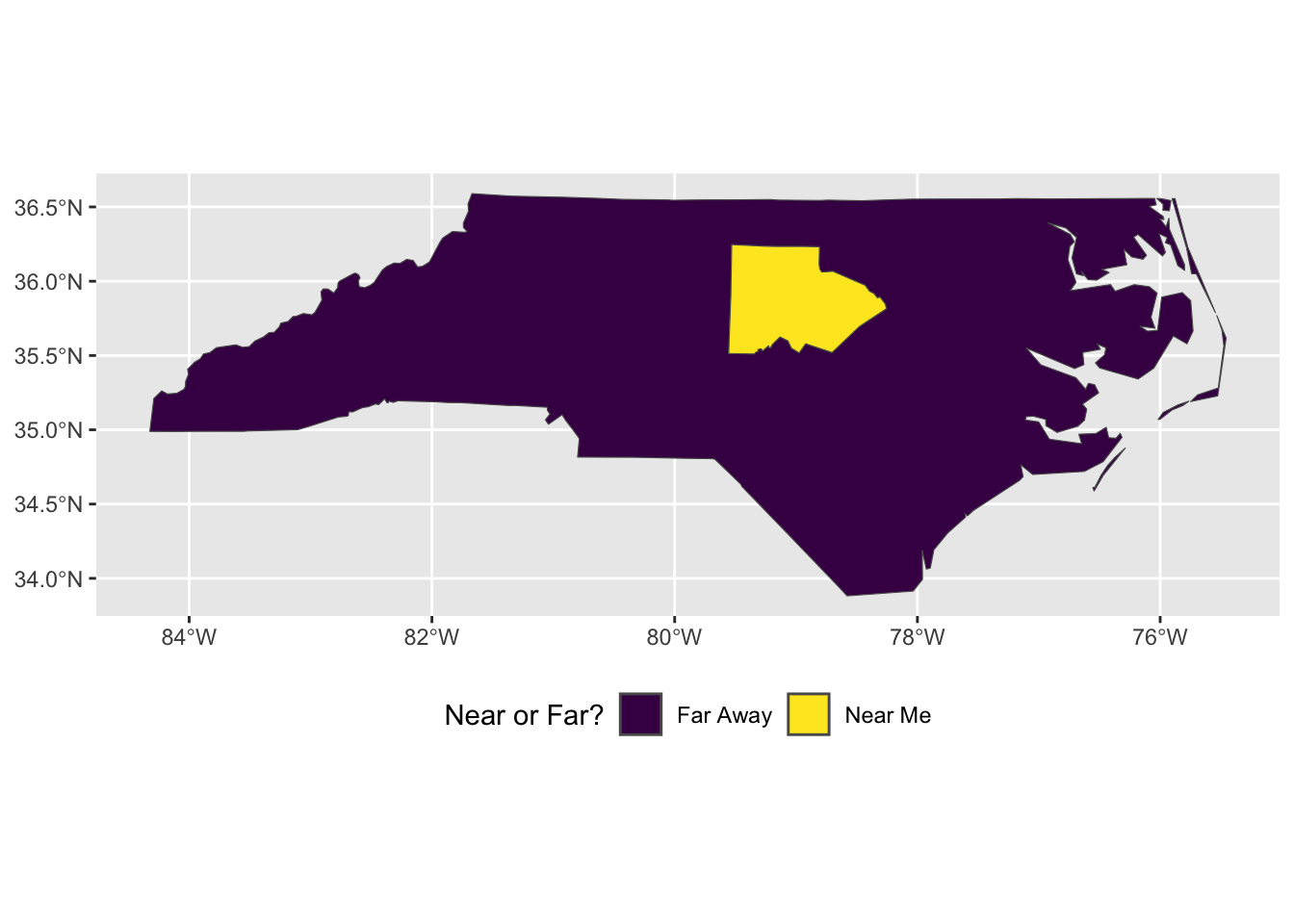
## Make a variable picking out five counties near where I livenc <- nc |>mutate(near_me =case_when(NAME %in%c("Orange", "Durham", "Wake", "Chatham", "Alamance") ~"Near Me", TRUE~"Far Away"))## What we just didnc |>count(near_me)
Simple feature collection with 2 features and 2 fields
Geometry type: GEOMETRY
Dimension:     XY
Bounding box:  xmin: -84.32385 ymin: 33.88199 xmax: -75.45698 ymax: 36.58965
Geodetic CRS:  NAD27
   near_me  n                       geometry
1 Far Away 95 MULTIPOLYGON (((-76.46926 3...
2  Near Me  5 POLYGON ((-79.54099 35.8369...
## These are all still county polygons. But now ...nc_merged <- nc |>group_by(near_me) |>summarize(mean_b =mean(BIR74), sum_sid =sum(SID74))nc_merged
Simple feature collection with 2 features and 3 fields
Geometry type: GEOMETRY
Dimension:     XY
Bounding box:  xmin: -84.32385 ymin: 33.88199 xmax: -75.45698 ymax: 36.58965
Geodetic CRS:  NAD27
# A tibble: 2 × 4
  near_me  mean_b sum_sid                                               geometry
  <chr>     <dbl>   <dbl>                                         <GEOMETRY [°]>
1 Far Away  3137.     616 MULTIPOLYGON (((-76.46926 34.69328, -76.2877 34.87701…
2 Near Me   6387.      51 POLYGON ((-79.54099 35.83699, -79.55536 35.51305, -79…
## Now we only have two polygonsnc_merged |>ggplot() +geom_sf(mapping =aes(fill = near_me)) +scale_fill_viridis_d() +theme(legend.position ="bottom") +labs(fill ="Near or Far?")
Source Code
---title: "Example 06: Maps"---## Setup```{r}library(here) # manage file pathslibrary(socviz) # data and some useful functionslibrary(tidyverse) # your friend and minelibrary(tidycensus) # Tidily interact with the US Censuslibrary(maps) # Some basic mapslibrary(sf) # Make maps in ggplotlibrary(tigris) # Talk to the Census's TIGER datalibrary(colorspace) # Paletteslibrary(nycdogs) # New York City dog license data```## Mapping ### Joining tables, and using `geom_polygon()`Remember, we use `geom_polygon()` as a kind of illustration of what's happening conceptually. It is not our go-to method for mapping. ```{r}# Create a theme that turns off most of the stuff ggplot usually printstheme_map <-function(base_size=9, base_family="") {require(grid)theme_bw(base_size=base_size, base_family=base_family) %+replace%theme(axis.line=element_blank(),axis.text=element_blank(),axis.ticks=element_blank(),axis.title=element_blank(),panel.background=element_blank(),panel.border=element_blank(),panel.grid=element_blank(),panel.spacing=unit(0, "lines"),plot.background=element_blank(),legend.position ="inside",legend.justification =c(0,0),legend.position.inside =c(0,0) )}head(county_map)dim(county_map)head(county_data)dim(county_data)county_full <-left_join(county_map, county_data, by ="id")p <-ggplot(data = county_full,mapping =aes(x = long, y = lat,fill = pop_dens, group = group))p1 <- p +geom_polygon(color ="gray70", size =0.1) +coord_equal()p2 <- p1 +scale_fill_brewer(palette="Blues",labels =c("0-10", "10-50", "50-100","100-500", "500-1,000","1,000-5,000", ">5,000"))p2 +labs(fill ="Population per\nsquare mile") +theme_map() +guides(fill =guide_legend(nrow =1)) +theme(legend.position ="bottom")```### Using simple features and `geom_sf()`The simple features model and associated `geom_sf()` is a much more compact and efficient way to draw maps.```{r}nyc_fb <- nyc_license |>group_by(zip_code, breed_rc) |>tally() |>mutate(freq = n /sum(n),pct =round(freq*100, 2)) |>filter(breed_rc =="French Bulldog")nyc_fbfb_map <-left_join(nyc_zips, nyc_fb)## A map theme for NYCtheme_nymap <-function(base_size=9, base_family="") {require(grid)theme_bw(base_size=base_size, base_family=base_family) %+replace%theme(axis.line=element_blank(),axis.text=element_blank(),axis.ticks=element_blank(),axis.title=element_blank(),panel.background=element_blank(),panel.border=element_blank(),panel.grid=element_blank(),panel.spacing=unit(0, "lines"),plot.background=element_blank(),legend.position ="inside",legend.justification =c(0,0),legend.position.inside =c(0.1, 0.6), legend.direction ="horizontal" )}fb_map |>select(zip_code, po_name, breed_rc:pct) |>pull(pct)``````{r}#| out-width: 100%#| fig-width: 10#| fig-height: 9fb_map |>filter(n >1) |>ggplot(mapping =aes(fill = pct)) +geom_sf(color ="gray80", size =0.1) +scale_fill_viridis_c(option ="A") +labs(fill ="Percent of All Licensed Dogs") +# This next bit is a hack--we're just positioning the boxes# relative to the latitude/longitude coordinatesannotate(geom ="text", x =-74.145+0.029, y =40.82-0.012, label ="New York City's French Bulldogs", size =6) +annotate(geom ="text", x =-74.1468+0.029, y =40.8075-0.012, label ="By Zip Code. Based on Licensing Data", size =5) +theme_nymap() +guides(fill =guide_legend(title.position ="top", label.position ="bottom",keywidth =1, nrow =1))```### Keeping zero-count rowsWe'll also fix the color here.```{r}nyc_license |>filter(extract_year ==2018) |>group_by(zip_code, breed_rc) |>tally() |>mutate(freq = n /sum(n),pct =round(freq*100, 2)) |>filter(breed_rc =="French Bulldog")nyc_fb <- nyc_license |>group_by(zip_code, breed_rc) |>tally() |>ungroup() |>complete(zip_code, breed_rc, fill =list(n =0)) |>mutate(freq = n /sum(n),pct =round(freq*100, 2)) |>filter(breed_rc =="French Bulldog")fb_map <-left_join(nyc_zips, nyc_fb)fb_map``````{r}#| out-width: 100%#| fig-width: 10#| fig-height: 9fb_map |>ggplot(mapping =aes(fill = pct)) +geom_sf(color ="gray80", size =0.1) +scale_fill_continuous_sequential(palette ="Oranges") +labs(fill ="Percent of All Licensed Dogs in the City") +annotate(geom ="text", x =-74.145+0.029, y =40.82-0.012, label ="New York City's French Bulldogs", size =6) +annotate(geom ="text", x =-74.1468+0.029, y =40.8075-0.012, label ="By Zip Code. Based on Licensing Data", size =5) +theme_nymap() +guides(fill =guide_legend(title.position ="top", label.position ="bottom",keywidth =1, nrow =1))```## Census data ### Population components example```{r}#| message: false#| results: hide# From the Census. You will need a census API key and the tidycensus packageus_components <-get_estimates(geography ="state", product ="components", vintage =2019)``````{r}us_componentsunique(us_components$variable)``````{r}#| message: false#| results: hidenet_migration <-get_estimates(geography ="county",variables ="RNETMIG",year =2019,geometry =TRUE,resolution ="20m") |>shift_geometry() # puts Alaska and Hawaii in the bottom left``````{r}order <-c("-15 and below", "-15 to -5", "-5 to +5", "+5 to +15", "+15 and up")net_migration <- net_migration |>mutate(groups =case_when( value >15~"+15 and up", value >5~"+5 to +15", value >-5~"-5 to +5", value >-15~"-15 to -5",TRUE~"-15 and below" )) |>mutate(groups =factor(groups, levels = order))net_migration``````{r}#| message: false#| results: hide#| out-width: 100%#| fig-width: 12#| fig-height: 9# So we can draw state boundaries (our migration data is at the county level)state_overlay <- tigris::states(cb =TRUE,resolution ="20m") |>filter(GEOID !="72") |>shift_geometry()ggplot() +geom_sf(data = net_migration, mapping =aes(fill = groups, color = groups), size =0.1) +geom_sf(data = state_overlay, fill =NA, color ="black", size =0.1) +scale_fill_brewer(palette ="PuOr", direction =-1) +scale_color_brewer(palette ="PuOr", direction =-1, guide ="none") +coord_sf(datum =NA) +theme_minimal() +labs(title ="Net migration per 1000 residents by county",subtitle ="US Census Bureau 2019 Population Estimates",fill ="Rate",caption ="Data acquired with the R tidycensus package")```## Simple Features work smoothly with dplyr grouping and summarizing ```{r}## This shapefile comes built-in to the sf package as an example. Here## we extract it and put it in an objectnc <-st_read(system.file("shape/nc.shp", package ="sf"), quiet = T)nc## Mapggplot(nc) +geom_sf()``````{r}## Make a variable picking out five counties near where I livenc <- nc |>mutate(near_me =case_when(NAME %in%c("Orange", "Durham", "Wake", "Chatham", "Alamance") ~"Near Me", TRUE~"Far Away"))## What we just didnc |>count(near_me)```Map it:```{r}nc |>ggplot() +geom_sf(mapping =aes(fill = near_me)) +scale_fill_viridis_d() +theme(legend.position ="bottom") +labs(fill ="Near or Far?")``````{r}## These are all still county polygons. But now ...nc_merged <- nc |>group_by(near_me) |>summarize(mean_b =mean(BIR74), sum_sid =sum(SID74))nc_merged## Now we only have two polygonsnc_merged |>ggplot() +geom_sf(mapping =aes(fill = near_me)) +scale_fill_viridis_d() +theme(legend.position ="bottom") +labs(fill ="Near or Far?")```